Classification of hand written letters or digits using Neural Network

Sofar we have learned how to run a simple tensorflow example in python. Today Iwill discuss the classification problem of hand written letters or digits usingNeural Network with a single hidden layer. Will also show accuracy comparison between logistic regression and neural network.
TensorFlow does all the work by itself and you will not understand anything if you are not familiar with the basic of Machine Learning techniques. I suppose you know the basics, lets proceed.
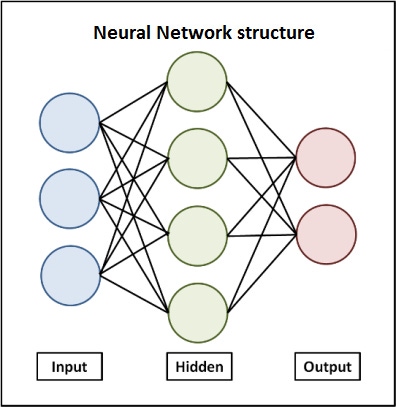
Neural Networks are the combination of linear and nonlinear techniques. The linear is the logistic regression used with an activation function (Non Linear) which can be Sigmoid or ReLu (Rectified Linear Unit), this activation function are also referred as the hidden layer(s) since the output of these cannot be observed. The below figure is the neural network structure with 2 NN layers and 1 hidden layers. From input to hidden there is a logistic function and same from hidden to output, while in hidden there is an activation.
Lets start with the python code, following are some of the functions needed to be explained.
Graphis a tensorflow core part, everything is dependent on the graph, so all variables, constants, statements that are set to be run on tensorflow needed to be in thegraph and upon training that graph must be explicitly mentioned so that thetraining could easily do what it wants.
graph= tf.Graph()
withgraph.as_default():
Using the above graph in session:
with tf.Session(graph=graph) as session:
Placeholder are just like Variable in tensorflow but with no initialization required, while Constant from the name are unchangeable
variables.tf_train_labels = tf.placeholder(tf.float32, shape=(batch_size, num_labels))
tf_valid_dataset = tf.constant(valid_dataset)
Neural_Network function does simply the logistic regression function and feeds its output to the relu function which further feeds hidden layer output to the final layer.
def Neural_Network(x, weights, biases):
    # Hidden layer with RELU activation
    layer_1 = tf.add(tf.matmul(x, weights['h1']), biases['b1'])
    hidden_layer = tf.nn.relu(layer_1)
    # Output layer with linear activation
    out_layer = tf.matmul(hidden_layer, weights['out']) + biases['out']
    return out_layer
Tocalculate the cost/loss:
loss= tf.reduce_mean(tf.nn.softmax_cross_entropy_with_logits(logits,tf_train_labels))
To optimize it and then minimize using a learning rate of 0.5:
optimizer= tf.train.GradientDescentOptimizer(0.5).minimize(loss)I have used Stochastic Gradient Descent (mini batch) rather than simple batch Gradient Descent because of its quickness in converging to the global minimum, SGD are very useful in deep learning. You can see that the batch size is mentioned and the loss is minimized by iterating over batches rather than the whole dataset.
Softmaxfunction converts the scores into probabilities.
train_prediction= tf.nn.softmax(logits)This is a 2 layer neural network with 1 hidden layer. Before you run it, you must download not MNIST.pickle file. This file contains 10,000 training, 500 validation and500 test datasets, each having 28x28 images of letters from (A to J) randomly shuffled (The same would work for digits). The pickle file is created so that it can be loaded in the memory easily. I assigned 3GB RAM to Ubuntu and this data size is enough, if you have more memory or want to try with different amount of data then you might need to create the pickle file yourselves. For help, I would prefer you to start Deep Learning course from Udacity, or you cango directly to this assignment to create your own pickle file.
Following is the full code, you can run directly using Jupyter Console. Run this from thepath of the notMNIST file. You might need to download several dependencies to run the code.
from __future__ import print_function
import numpy as np
import tensorflow as tf
from six.moves import cPickle as pickle
from six.moves import range

pickle_file = 'notMNIST.pickle'

with open(pickle_file, 'rb') as f:
  save = pickle.load(f)
  train_dataset = save['train_dataset']
  train_labels = save['train_labels']
  valid_dataset = save['valid_dataset']
  valid_labels = save['valid_labels']
  test_dataset = save['test_dataset']
  test_labels = save['test_labels']
  del save  # hint to help gc free up memory
  print('Training set', train_dataset.shape, train_labels.shape)
  print('Validation set', valid_dataset.shape, valid_labels.shape)
  print('Test set', test_dataset.shape, test_labels.shape)

image_size = 28
num_labels = 10

def reformat(dataset, labels):
  dataset = dataset.reshape((-1, image_size * image_size)).astype(np.float32)
  # Map 0 to [1.0, 0.0, 0.0 ...], 1 to [0.0, 1.0, 0.0 ...]
  labels = (np.arange(num_labels) == labels[:,None]).astype(np.float32)
  return dataset, labels
train_dataset, train_labels = reformat(train_dataset, train_labels)
valid_dataset, valid_labels = reformat(valid_dataset, valid_labels)
test_dataset, test_labels = reformat(test_dataset, test_labels)
print('Training set', train_dataset.shape, train_labels.shape)
print('Validation set', valid_dataset.shape, valid_labels.shape)
print('Test set', test_dataset.shape, test_labels.shape)

# With gradient descent training, even this much data is prohibitive.
# Subset the training data for faster turnaround.
train_subset = 10000
batch_size = 100

def Neural_Network(x, weights, biases):
    # Hidden layer with RELU activation
    layer_1 = tf.add(tf.matmul(x, weights['h1']), biases['b1'])
    hidden_layer = tf.nn.relu(layer_1)
    # Output layer with linear activation
    out_layer = tf.matmul(hidden_layer, weights['out']) + biases['out']
    return out_layer

graph = tf.Graph()
with graph.as_default():

  # Input data. For the training data, we use a placeholder that will be fed
  # at run time with a training minibatch.
  tf_train_dataset = tf.placeholder(tf.float32, shape=(batch_size, image_size * image_size))
  tf_train_labels = tf.placeholder(tf.float32, shape=(batch_size, num_labels))
  tf_valid_dataset = tf.constant(valid_dataset)
  tf_test_dataset = tf.constant(test_dataset)

  n_hidden_1 = 1024 # 1st layer number of features
  n_input = 784 # MNIST data input (img shape: 28*28)
  n_classes = 10 # MNIST total classes (0-9 digits)
  # Training computation.

  #Store layers weight & bias
  weights = {
    'h1': tf.Variable(tf.random_normal([n_input, n_hidden_1])),
    'out': tf.Variable(tf.random_normal([n_hidden_1, n_classes]))
  }
  biases = {
    'b1': tf.Variable(tf.random_normal([n_hidden_1])),
    'out': tf.Variable(tf.random_normal([n_classes]))
  }

# Construct model
  logits = Neural_Network(tf_train_dataset, weights, biases)

  loss = tf.reduce_mean(tf.nn.softmax_cross_entropy_with_logits(logits, tf_train_labels))

  # Optimizer.
  optimizer = tf.train.GradientDescentOptimizer(0.5).minimize(loss)

  # Predictions for the training, validation, and test data.
  train_prediction = tf.nn.softmax(logits)
  logits1 = Neural_Network(tf_valid_dataset, weights, biases)
  valid_prediction = tf.nn.softmax(logits1)
  logits2 = Neural_Network(tf_test_dataset, weights, biases)
  test_prediction = tf.nn.softmax(logits2)

num_steps = 801

def accuracy(predictions, labels):
  return (100.0 * np.sum(np.argmax(predictions, 1) == np.argmax(labels, 1))
          / predictions.shape[0])

with tf.Session(graph=graph) as session:
  tf.global_variables_initializer().run()
  print("Initialized")
  for step in range(num_steps):
    # Pick an offset within the training data, which has been randomized.
    # Note: we could use better randomization across epochs.
    offset = (step * batch_size) % (train_labels.shape[0] - batch_size)
    # Generate a minibatch.
    batch_data = train_dataset[offset:(offset + batch_size), :]
    batch_labels = train_labels[offset:(offset + batch_size), :]
    # Prepare a dictionary telling the session where to feed the minibatch.
    # The key of the dictionary is the placeholder node of the graph to be fed,
    # and the value is the numpy array to feed to it.
    feed_dict = {tf_train_dataset : batch_data, tf_train_labels : batch_labels}
    _, l, predictions = session.run(
      [optimizer, loss, train_prediction], feed_dict=feed_dict)
    if (step % 500 == 0):
      print("Minibatch loss at step %d: %f" % (step, l))
      print("Minibatch accuracy: %.1f%%" % accuracy(predictions, batch_labels))
      print("Validation accuracy: %.1f%%" % accuracy(
        valid_prediction.eval(), valid_labels))
      #print(weights['out'].eval())
  print("Test accuracy: %.1f%%" % accuracy(test_prediction.eval(), test_labels))
Also available on my Github repo.
I have already mentioned in the past that I would not go in detail of each of thefunction since it is already present at the official website of TensorFlow, myfocus is to discuss the problems that most of the people usually face whileusing tensorflow.
One of the question I had was Why cannot Logistic Regression classify the hand written problems? Handwritten letters or digits classification is difficult to solve using linear approaches because of its non-linearity. To deal with non-linearity there will be the addition of thousands of extra features in the logistic regression equation to represent the high polynomial degree which will try to fit it perfectly. You can try it but you will see a great difference in the accuracy as compared to neural networks.
The code can be customized easily, only few lines of code needs to be changed. Replace the weights and biases with the following:
 weights = tf.Variable(tf.truncated_normal([image_size * image_size, num_labels]))
 biases = tf.Variable(tf.zeros([num_labels]))
Change the Neural Network function to this:
 def Neural_Network(x, weights, biases):
    layer_1 = tf.add(tf.matmul(x, weights['h1']), biases['b1'])
    return layer_1
I got around 87% from this and 91% from neural network, that seems to be a great improvement. Let me know how much accuracy you got from both of the versions. You might get different in case you make your own pickle.
In the next part I will introduce the regularization techniques to overcome overfitting issues in neural network which will further increase the accuracy.


