Analyzing WhatsApp Group Chat Using R

In this blog post, you will learn how to do WhatsApp Group Chat analyzes using R programming language. Analyzing friends’ messages and their behavior is quite interesting. You will see simple but useful visualization using ggplot2 at the end of this post.

We will follow the following steps to carry out our analysis.

• Data Collection

• Data Wrangling

• Feature Engineering

• Visualization

You will also need to install and load several R packages to achieve this task,check full code available on Github.

Data Collection

The first and the basic step is to collect the data, in our scenario you can usethe WhatsApp feature to email the chat. Open the chat, go to options, thenmore, you will find email chat feature. You can email the chat without the media but it does not mean that it will remove all the messages that contain media, it will online replace it with a simple text <Media omitted>.

Once downloaded on your PC, you can see it is a raw text file. Lets load the datawith the help of following command.

all_data= readLines('whatsap_friends.txt')

Data Wrangling

As discussed many times previously, data wrangling or cleaning is one of the most important part of data analyses because it takes more than 60% of the total time of the process.

We have to parse the file and extract useful information in the form of dataframe. The file contains the data in the following format: Date, time – Sender: message

Before diving deep, let me give you a brief idea of what we are going to do in this phase.

1. Separate data and time

2. Set temporary value to sender

3. Set each line from raw file to the message column, contains the whole format as above.

4. Extract all messages that have date, time set, that is complete cases.

5. Extract sender names from messages and set to sender column.

6. Remove date and time from message.

We have used str_trim() functionf rom stringr package, the purpose of this function is to remove the whitespaces from both ends.

The date and time format needs to be adjusted, its based on your timezone, so check out your format and see what format does it follow and change the following code accordingly.

#Extracting date and time 
date_time <- format(strptime(all_data, "%m/%d/%y, %I:%M %p"),"%m/%d/%y, %H:%M")
#Extracting date
date = gsub(",.*$","",date_time) #Fetching all before ","

#Extracting time
time = gsub("^.*,","",date_time) #Fetching all after ","
time = str_trim(time)

sender <- 'sender' #Temorary Data
message <- all_data

Now we have extracted date and time, we can make a dataframe.

clean_data= data.frame(date,time,sender,message)

The data is not yet cleaned, we will make clean_data really clean with the following commands.

#Extracting sender and message from the data frame
#Fetching all the data with complete cases from the fourth column
sender_message = clean_data[complete.cases(clean_data),4]
sender_message = gsub("^.*?-","",sender_message)
sender_message = str_trim(sender_message)
#Extracting message
message = gsub("^.*?:","",sender_message)
message = str_trim(message)

#Updating the data frame with new message data
clean_data$message <- as.character(clean_data$message)
clean_data[complete.cases(clean_data),4] <- message

#Extracting sender names
sender = gsub("?:.*$","",sender_message)
sender = str_trim(sender)
#Updating the data frame with new sender data
clean_data$sender <- as.character(clean_data$sender)
clean_data[complete.cases(clean_data),3] <- sender

Now you have adjusted all the variables’ values in their columns but the one final problem is still left, which you might have seen in the raw file, whenever a sender sends consecutive messages then it contain date, time and sender name only for the first, we have to fill all that out.

For Example, if Michael sends three messages in a row, it will be like:

07/28/17,12:00 AM – Michael: HI!
How are you?
Where are you?

So we have to add the date, time and sender name to the two last records. We cando that using the transform function from the Zoo package, it will fill out allthe NA values with the previous values.

clean_data<- transform(clean_data, date = na.locf(date), time = na.locf(time),                        sender =na.locf(sender))

You can also use custom functions like if you have unknown contacts, you can remove them. Also, we have kept all the messages that represent media, you may remove them. Now we can see the data is cleaned and we can proceed with our next steps, use view and summary function:

view(clean_data)
summary(clean_data)

Feature Engineering

Featureengineering is one of the most creative part of data analysis, it is of greatuse especially when using statistical models but in our case we know a single feature can help us to visualize the data more efficiently in future.

We know message length can prove to be a great feature, but we also know that media messages represent <Media omitted> which are of 15 characters but of no use since its the replacement of the actual media, we need to keep media length to 0, so lets create:

#Setting media messages to empty space for length 0
clean_data[clean_data=="<Media omitted>"]<-""
#Finding length of each message
clean_data$message_length <- nchar(clean_data$message)
#Restting media messages 
clean_data[clean_data==""]<-"<Media omitted>"
summary(clean_data$message_length)

Data Visualization

Now lets plot some basic bar graphs using the mighty ggplot package.

ggplot(clean_data,aes(sender))+  geom_bar()+  ylab('number of messages')

ggplot(clean_data,aes(sender,message_length))+  geom_bar(stat='identity')+  ylab('sum of message length')

Now plotting mean message length across each sender. We will need to use aggregation function to find the mean.

grouped_mean_length <- aggregate(message_length ~ sender, clean_data, mean)

ggplot(grouped_mean_length, aes(sender,message_length))+
  geom_bar(stat="identity")+
  ylab("mean of message length")

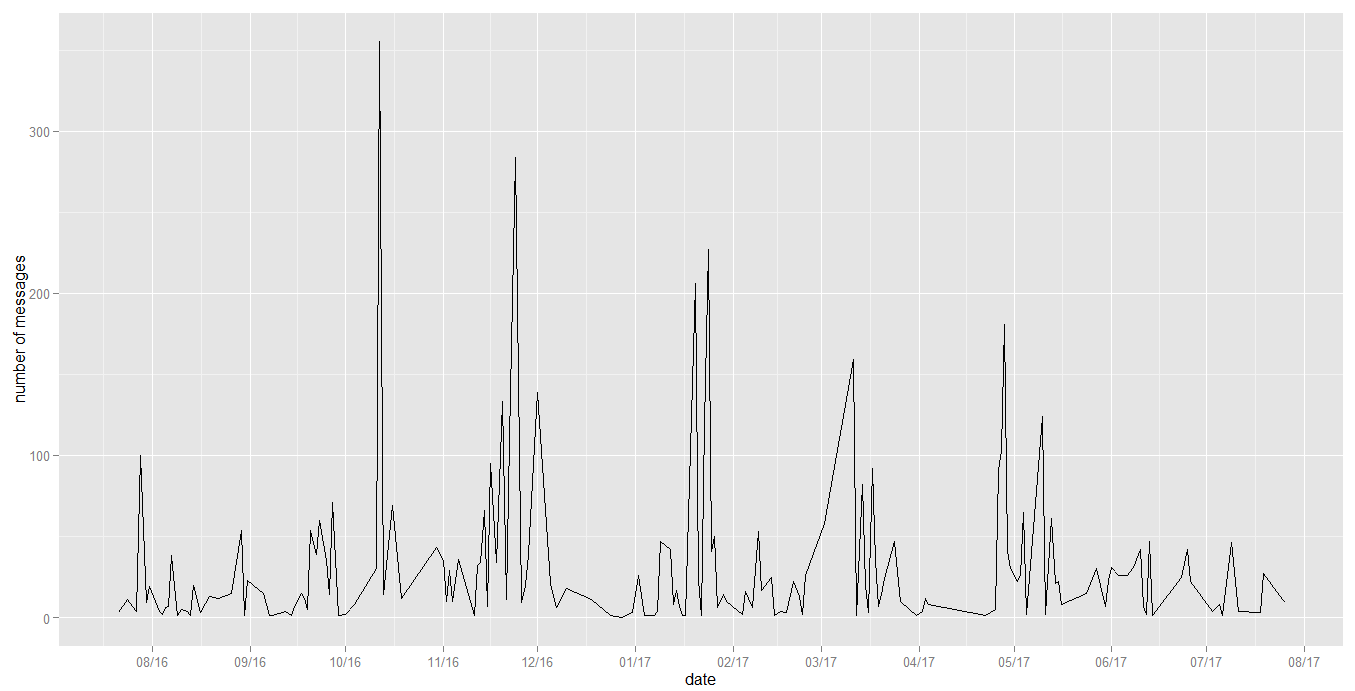
Lets make a little complex plot, we need to plot date vs number of records, we can use the table function to create a new data frame.

date_count<-data.frame(table(clean_data$date))
colnames(date_count) <- c('date', 'count')

Now lets make a scatter plot, scale_x_date is a function available in scales package, it will help us in axis scaling.

Note: Date strings must be converted to dates using as.Date()

#Scatter plot for the number of messages per given date
ggplot(date_count, aes(as.Date(date, "%m/%d/%y"),count))+
  geom_line()+
  scale_x_date(breaks = date_breaks("1 months"),labels = date_format("%m/%y"))+
  xlab("date")+
  ylab("number of messages")

You can get the full code at the Github.

You might have noticed that we have not carried out any Data Science stuff, we only did the data analysis, I will try to do some sentiment analysis on the messages, will try to classify kind of messages with respect to the sender.  So stay tuned!