Machine Learning on Titanic Dataset using R

After performing some data analysis on Football News Guru Data using R, I came back to one of the most fundamental dataset extracted from the Titanic disaster, you can find it on Kaggle from the name Titanic: Machine Learning from Disaster. The purpose of this article is to extent the Data Science Dojo Tutorial to increase the accuracy of the model.

On Kaggle you might see people getting 100 percent accuracy which is quite impossible and is probably done through cheating.

In this article, I will not tell everything step by step since you can find the Data Science Dojo tutorial here, if you are new you must go through that tutorial its really interesting.

To improve the accuracy, I combined my techniques to the code provided by Data Science Dojo vice president David Langer to increase the accuracy by 2%.

I added two things in the code to improve the accuracy, one I engineered a new feature named Title and second I used transformation technique on the Fare variable in order to reduce the variance.

I thought engineering a new feature from the variable Name can be useful because the outcome Survived can be partially dependent on the Name title in some way, so following code does what I wanted, extracted the titles into new feature named Title, then converted all less occurring features into the common features like some French female titles into Lady and similarly some male titles into Sir.

#Modification (New Feature named Title introduced from Names)
train$Name <- as.character(train$Name)
strsplit(train$Name[1], split='[,.]')
strsplit(train$Name[1], split='[,.]')[[1]]
strsplit(train$Name[1], split='[,.]')[[1]][2]
train$Title <- sapply(train$Name, FUN=function(x) {strsplit(x, split='[,.]')[[1]][2]})
train$Title <- sub(' ', '', train$Title)
table(train$Title)

#Converting less occurring titles into common titles
train$Title[train$Title %in% c('Capt', 'Don', 'Major', 'Col')] <- 'Sir'
train$Title[train$Title %in% c('Dona', 'Lady', 'the Countess', 'Jonkheer',
                               'Mlle', 'Mme', 'Ms')] <- 'Lady'

Also, I added the following code to convert the newly generated feature into categorical variable.

train$Title<- as.factor(train$Title)

Second is the log transformation on Fare. Since I observed that the Fare variable plot is skewed, I simply took a log which reduced its skewness as well as variance, thus increasing accuracy.

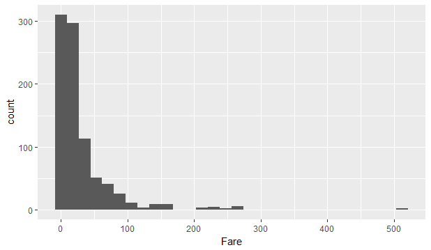
Fare histogram plot without transformation

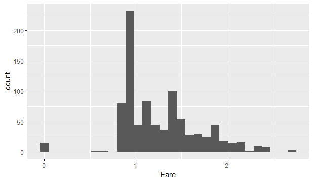
Fare histogram plot with log transformation

#Taking log10 for the feature Fare
train$Fare<- ifelse(train$Fare !=0,  log10(train$Fare), 0)

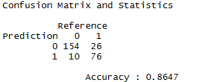
From the last line in the full code version, we generated a confusion matric.

confusionMatrix(preds,titanic.test$Survived) 

It gives a confusion matrix along with many other important quantities like Accuracy. The accuracy might slightly differ when you rerun it on your machine because of the automated process, but the accuracy lies between 86.2 and 87.2 percent.

You can find the full code at my Github repository.

Would love to get a feedback, any suggestion for further improvement or any mistake that you identified. Comment below!